Sound of the handpan: analysis and synthesis

---

No File

1. Background

The handpan is a type of percussive musical instrument made from two hemispherical shells of nitrided steel, connected together along their circular rim. The upper shell contains at least eight harmonically tuned note-fields, one of which (the Ding) is positioned at the centre, with the remaining note-fields arranged around it in a circular pattern. A note-field typically has an elliptical shape with a convex or concave dimple. The bottom shell is a smooth surface with a single central opening (the Gu), functioning as the neck of the Helmholtz resonator formed by the enclosed air cavity inside the body [1]. Figure 1 shows a typical handpan from both sides.

The instrument produces sound primarily through the vibration of its own body when struck, therefore it’s categorized as a directly struck idiophone under the Hornbostel–Sachs system [2]. Its design evolved from the steelpan, the distinctive Caribbean instrument developed in Trinidad and Tobago during the 1950’s from repurposed WWII oil barrels [3]. The Hang, introduced by Felix Rohner and Sabine Schärer in 2001, is considered the first example of this instrument type [3], [4], [5].

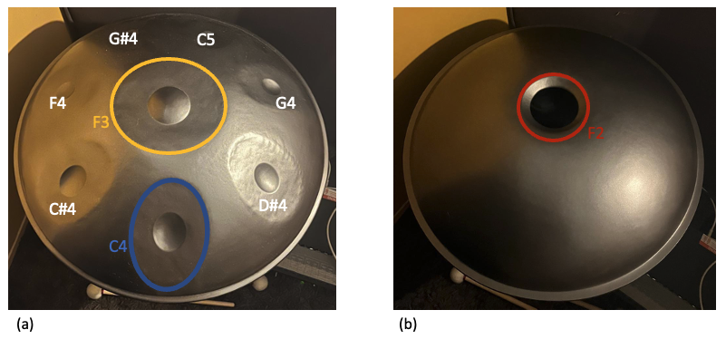
Figure 1: Handpan under study with (a) Ding side and (b) Gu side.

2. Sound production mechanisms

Governing physical principles
The instrument’s sound production mechanisms are mainly governed by:

1. vibration of the instrument body when struck: the shell and harmonically tuned note-fields vibrate and radiate sound,

2. radiation by the Helmholtz resonator formed by the air column in the Gu, backed by the air cavity inside the body,

3. coupling between the different note-fields and resonator.

Each note-field is tuned to a note within a musical scale and mainly produces harmonics with approximate ratio 1:2:3, corresponding to a fundamental frequency f₀, an octave (f₁ = 2f₀) and a compound perfect fifth (f₂ = 3f₀). Higher-order harmonics are also produced but weaker in amplitude and not individually tuned, nevertheless contributing to the instrument’s timbre [1].

Every harmonic generated by a note-field corresponds to one of its vibrational modes. In case of a tuned note-field, the fundamental f₀ corresponds to mode (0,1), f₁ to mode (1,1)_a and f₂ to mode (1,1)_b [1]. This is not necessarily the case for untuned elliptical plates [6], [7]. By skilfully hammering and shaping the material, which introduces compressive in-plane stresses producing buckling phenomena (wrinkles) in the note-field (see Figure 1), the eigenfrequencies of the (0,1), (1,1)_a, and (1,1)_b modes are aligned with the 1:2:3 harmonic ratio [8].

From this follows that different harmonics can be selectively emphasised or supressed by striking or damping the note-field in specific areas. Striking the ‘D-sweetspot’ mainly excites the fundamental, whereas striking the note-field along the nodal lines of mode (1,1)_a or (1,1)_b respectively supresses the 2nd or 3rd harmonic [8]. This is shown schematically in Figure 2.

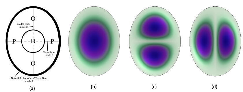
Figure 2: (a) Note-field sweetspots and nodal lines, adapted from [9] with D: mode (0,1) sweetspot (f), O: mode (1,1)_a sweetspot (2f) and P: mode (1,1)_b sweetspot (3f). (b) modeshape (0,1), (c) modeshape (1,1)_a and (d) modeshape (1,1)_b.

Typically, the handpan is played by hand by means of percussive strikes. Striking a note-field area mainly excites its harmonics, producing a sound with a well-defined pitch. Alternatively, the instrument might be struck in between note-fields, generating a percussive, dissonant sound with a metallic timbre and ill-defined pitch due to many anharmonic partials being excited. Other playing techniques may include exciting the Gu directly, or inducing vibrato by pressing the shell [8].

Due to coupling between the note-fields and the air cavity, exciting the handpan yields a rich sound, composed of more harmonics than only those produced by the struck note-field [4]. Beating may be introduced due to small imperfections in tuning between the different note-fields.

Figure 3 shows holographic interferograms of a handpan driven at small and large amplitude around the first three harmonics of its Ding (F3), showing excitation of non-directly struck note-fields with modal frequencies close to the driving frequency. In this case, at a driving frequency of 520 Hz (F3-f₂), resonance of the (1,1)_a mode of the C4 note-field is observed, corresponding to its 2nd harmonic (C4-f₁ = 523.2 Hz) [1].

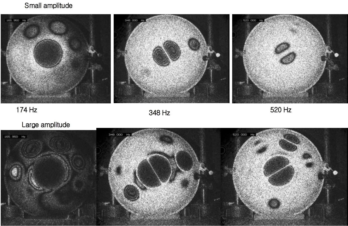
Figure 3: Coupling between note-fields. Image taken from [8], originally from [1].

Modes of vibration of a note-field
The fundamental frequency f₀ (in Hz) related to mode (0,1) of an isotropic elliptical plate with uniform thickness is approximated analytically by [9]

$$f_0\approx \frac{0.291c_{L}h}{a^2}\sqrt{1+\frac{2}{3}{\left(\frac{a}{b}\right)}^2+{\left(\frac{a}{b}\right)}^4}$$ (1)

where h is the thickness of the plate (in m), and a and b are the semimajor and semiminor axes of the ellipse (in m). The quasi-longitudinal wave velocity c _L in an infinite plate (in m/s) is given by [9]

$$c_L=\sqrt{\frac{E}{\rho (1-{\nu }^2)}}$$ (2)

with ρ the density (in kg/m³) and ν the Poisson ratio. For the handpan under study, this model closely matches theoretical frequencies of the note-fields’ fundamental frequencies, as illustrated in Table 1. A thickness of h = 0.5 mm for the shell is assumed in accordance with f_0,th of the C4 note-field.

Table 1: Analytic approximation of fundamental frequencies of elliptical plates with uniform thickness. f_0,model from Eq. 1, f_0,th from [10]. Dimensions are measured from the handpan under study. ϵ = (f_0,model – f_0,th)/f_0,th.

Note field	2a (m)	2b (m)	b/a	f0,model (Hz)	f0,th (Hz)	ϵ
F3	0.185	0.17	0.92	166	174.6	−0.05
C4	0.17	0.125	0.74	261.64	261.6	0.00
C#4	0.16	0.12	0.75	287.2	277.2	0.04
D#4	0.16	0.115	0.72	305.22	311.1	−0.02
F4	0.145	0.11	0.76	344.15	349.2	−0.01
G4	0.145	0.10	0.69	395.05	392	0.01
G#4	0.14	0.095	0.68	434.26	415.3	0.05
C5	0.12	0.085	0.71	554.33	523.3	0.06

Studies by Reddy et al. [7] and Singh and Chakraverty [6] report that the modal frequencies of modes (1,1)_a and (1,1)_b, relative to the eigenfrequency of mode (0,1), depend strongly on the eccentricity b/a of the ellipse. For b/a = 0.8, mode (1,1)_a approaches the desired harmonic ratio of 2:1, with a ratio f_11a/f₀₁ of 1.84. In contrast, mode (1,1)_b has a ratio f_11b/f₀₁ of 2.29, deviating largely from the target ratio 3:1 [7].

Results from a limited COMSOL eigenfrequency FEM study, carried out on a flat elliptical plate with uniform thickness and dimensions matching the C4 note-field supports these findings, as illustrated in Table 2.

Table 2: text

Table 2: Ratio of modal frequencies f_11a and f_11b over f01.

Source	b/a	f11a / f01	f11b / f01
Lakshmi Reddy [7]	0.8	1.8417	2.29
COMSOL	0.74	1.7546	2.35

This analysis illustrates the intricacies of the tuning process. Material properties, geometric shaping and the craft of controlled hammering are deterministic for a note-field’s final tuning. Both the analytical formulation and the literature demonstrate how parameters such as eccentricity and thickness affect the eigenfrequencies, and how aligning the specific modal frequencies with a 1:2:3 ratio is non-trivial. The discussed parameters represent only a subset of the many factors involved, demonstrating why the tuning of a note-field is often regarded an art.

3. Analysis

Methodology
Three recordings were made from a handpan tuned to an F minor scale by striking the C4 note-field at its D-sweetspot with a felt mallet. The first two notes were produced with a clean mallet rebound, allowing it to ring freely, struck gently and hard. The third note was produced with a similarly hard strike with the mallet left resting on the note-field. Recordings were made at a distance of approx. 20 cm in a dry environment to minimise room colouration. The notes were captured using a Behringer ECM8000 microphone and Focusrite Saffire interface, at 44.1 kHz sample rate. Leading and trailing silences were trimmed. Figure 4 shows the recording setup and microphone’s frequency response.

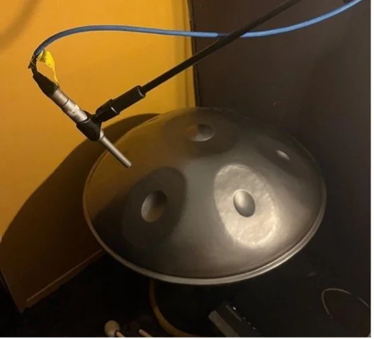
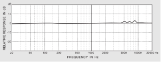
Figure 4: Picture of recording setup (left), and Frequency response of the ECM8000 [11] (right).

A frequency-domain analysis was carried out in MATLAB using the power spectral density (PSD) estimated via Welch’s method, using eight averages and Hamming windowing (Δf = 1.35 Hz for all recordings) [12], [13]. Partials and their amplitude are identified with a peak-finding algorithm and attributed to one of the eight note-fields. To account for imperfections in tuning, a tolerance of ±3% around the theoretical frequencies was applied [10]. The highest resonant peak within this range was identified as the corresponding harmonic. A similar methodology was used to identify the instrument’s Helmholtz resonant frequency. An initial time-domain analysis was carried with the Voicebox v_spgrambw spectrogram function [14]. This MATLAB function computes a STFT [15] on successive blocks of the time-varying signal, showing the signal’s spectrum over time. Additionally, a Hilbert transform was applied to obtain the instantaneous frequency and amplitude envelope of the harmonics of the struck note-field. The transform generally performs poorly on multicomponent signals [16]. Therefore, a set of very narrow bandpass FIR filters, centred at each measured harmonic, is applied to the signal. This forges quasi-monocomponent signals, enabling extraction of amplitude envelope and instantaneous frequency of spectral components, allowing for more intricate analysis. Results may become noisy if the signal is not sufficiently monocomponent.

Frequency domain analysis
Figure 5 shows the PSD of the first recording. The first four harmonics of the excited note-field (C4) are dominant in the spectrum. The measured Helmholtz resonance around 85 Hz agrees well with the analytic estimation of 86.8 Hz, obtained by [17]

$$f_{\text{HH,model}}=\frac{c}{2\pi }\sqrt{\frac{S}{(L_1+2\delta a)V}}$$ (3)

with c the speed of sound in air (343 m/s), a the radius (in m) and S the surface (in m²) of the Gu, L₁the neck length (in m) and δ the end correction to account radiation impedance of the hole (δ = 0.85, [17]). The volume V (in m³) of the air cavity was obtained from a CAD model of the examined handpan. The Helmholtz resonance corresponds with the fundamental frequency of an F2 note (87.3 Hz, [10]).

Most of the dominant harmonics can be attributed to the struck note-field (C4). Contrary, the third harmonic of G4 (1165 Hz) is strongly excited, although it is an anharmonic of C4. This suggests strong coupling between the C4 and G4 note-fields. This is further supported by the third harmonic of C4 (f₂) coinciding with the second harmonic of G4 (785 Hz). The coupling might be further facilitated by the 3:2 ratio (perfect 5th) between their fundamentals. The prominent peak at 1165 Hz could be interpreted as a manifestation of the ease of energy transfer between the two note-fields. Other coinciding harmonics, such as f₁ with the fundamental of C5, and f₃ with its second harmonic, suggest strong coupling between these note-fields as well. Attributing fractions of partials in the PSD to separate note-fields would require isolated recordings, which is outside the scope of this work.

Overall, the spectrum shows a small number of peaks with relatively high amplitude, most of which are integer multiples of the struck note-field’s fundamental. This indicates a consonant timbre, which agrees well with subjective findings from listening to the recording.

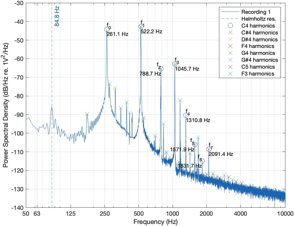
Figure 5: PSD of recording 1, over a limited frequency range to enhance visibility.

Figure 6 shows the PSD of the second, stronger strike of the C4 note-field. The most notable feature is the increase in number of peaks and their amplitude relative to f₀, especially in the region above f₃, indicating that the instrument ‘opens up’. The effect is observed for both harmonics and non-integer partials of the fundamental. This indicates that the instrument produces a sound that is brighter and more dissonant when excited with greater force. This finding agrees well with subjective experience. A detailed analysis of this nonlinear behaviour is beyond the scope of this work, however, it can be partly attributed to coupling between notes, which is nonlinear in character [9].

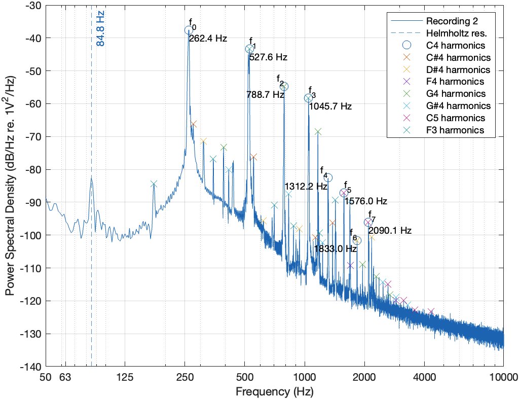
Figure 6: PSD of recording 2.

Figure 7 shows the PSD of the third recording. The amplitude of the fundamental (f₀) is reduced due to damping introduced by the resting mallet. It’s left on the D sweetspot, which corresponds with the antinode of the note-field’s mode (0,1), related to the fundamental. The amplitude of the third harmonic (f₂) has decreased, suggesting that it does not relate solely to mode (1,1)_b. Since the D-sweetspot lies on the mode’s nodal line, only little damping would be expected.

In contrast, amplitudes of f₁ and f₃ have not decreased significantly, explained by the D sweetspot coinciding with the nodal line of the corresponding modes (mode (1,1)_a and possibly (1,1)_b). Therefore, the resting mallet introduces little damping to these modes.

The Helmholtz resonance has shifted upwards to approximately 90 Hz, due to a reduced compliance of the air cavity inside the body; the resting mallet slightly increases the stiffness of the system, thereby increasing its resonant frequency. Finally, the spectrum shows a further increase in number and amplitude of anharmonic partials, consistent with the more dissonant sound and metallic timbre perceived in this recording.

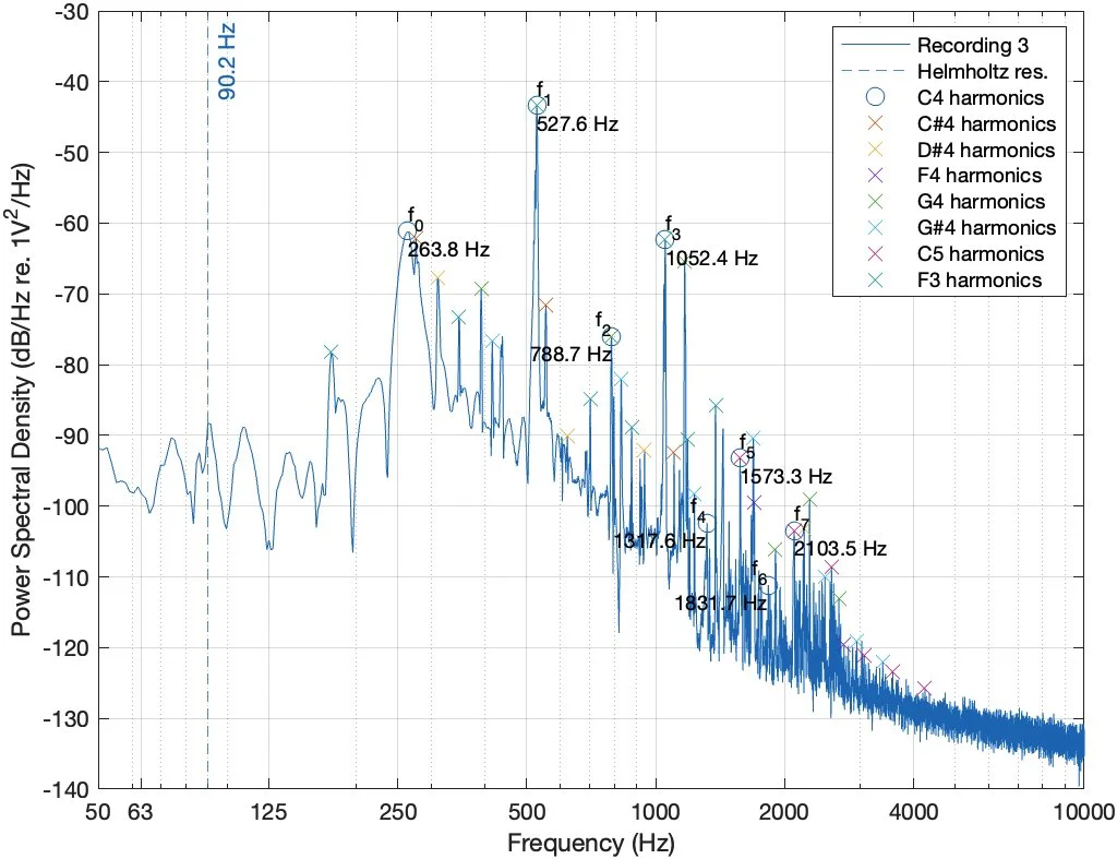
Figure 7: PSD of recording 3.

Time domain analysis
Figure 8a, 8c and 8e show the normalized time-varying spectral density for all three recordings over their full duration. Figure 8b, 8d and 8f present the first 150 ms of the corresponding spectrograms, scaled to power per decade to improve visibility of higher harmonics [18]. Figure 9a–f shows the amplitude envelope of the first five harmonics of the struck note-field, extracted using the Hilbert transform.

Consistent with the findings in the frequency analysis, increasing the striking force yields a nonlinear increase in amplitude of both higher harmonics and partials, notably in the frequency regions between f₃–f₄, f₄–f₅, and f₅–f₆. The increased damping and shorter decay time shown in Figure 8c and 8e is consistent with the increase in bandwidth of f₀ illustrated in Figure 6 and 7.

Figure 8b, 8d and 8f also illustrate that higher harmonics reach peak amplitude more slowly, which illustrates the ‘blooming’ sound of the instrument. While literature does not explain this phenomenon for handpans specifically, personal experience from playing the instrument showed that the third harmonic of the G4 note-field (1165 Hz) has a noticeably longer attack when excited indirectly via coupling than by directly striking the G4 note-field. This supports the notion that harmonics require time to developed when excited via coupling. A similar effect is reported for other directly struck metal idiophones, like the gong and cymbal [9], [19].

Furthermore, beating is observed, most prominent for the second harmonic of the struck note-field (f₁), and increases with striking force, as seen in Figure 8a and 8c, and Figure 9a and 9c. This likely arises from small tuning deviations between the C4, C5 and F3 note-fields with their respective second, first and fourth harmonics around 520 Hz interfering and introducing amplitude modulation.

Finally, Figure 8e shows that resting the mallet on the D-sweetspot results in a decrease in decay time for the struck note-field’s harmonics, most notably f₀ and f₂, and to a lesser extent f₁ and f₃. This agrees with findings in the frequency analysis, showing a decrease in amplitude for f₀ and f₂ – and to a lesser extent for f₁ and f₃ – due to resting the mallet. It should be noted that resting the mallet also reduces the decay time of the third harmonic of the coupled G4 note-field (1165 Hz), indicating that decay time is influenced by coupling as well. The fast beating at f₁ for the damped note likely results from interaction between the shell and the mallet, since it was left resting on the note-field – not pushed against it. As a result, the mallet lifts off periodically due to the shell’s displacement, thus damping the shell’s vibration periodically.

(a)

(b)

(c)

(d)

(e)

(f)

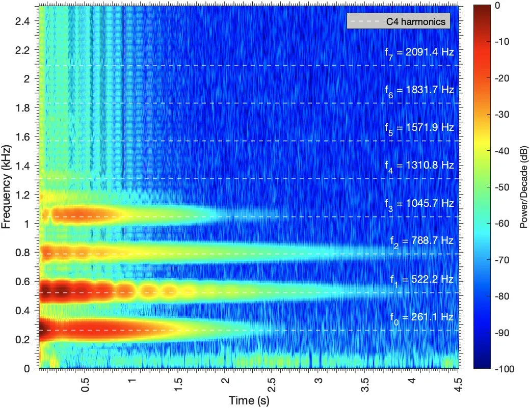
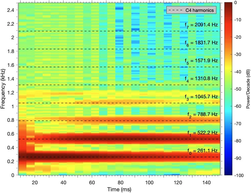
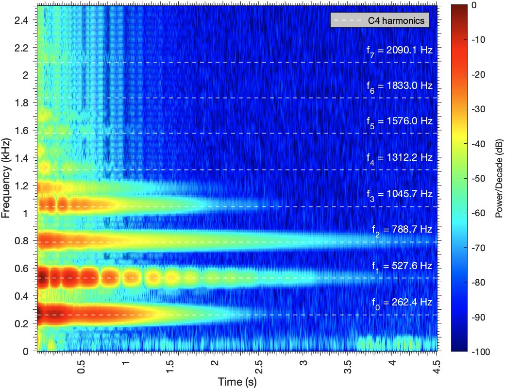
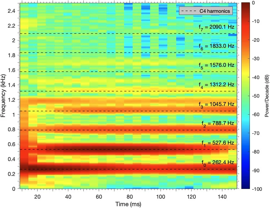
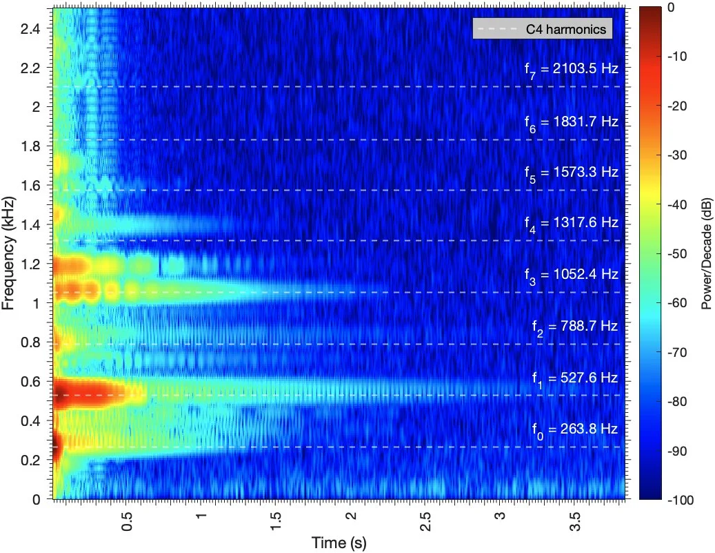
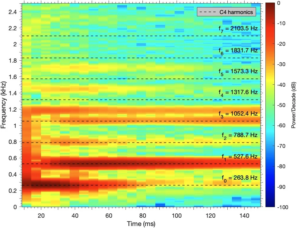
Figure 8: Normalised spectrograms for the three recordings (top, middle, bottom), over their full length (left), and the first 150 ms after impact (right).

(a)

(b)

(c)

(d)

(e)

(f)

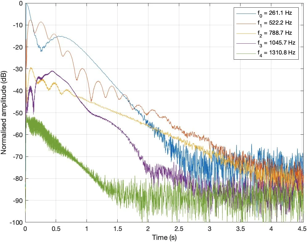
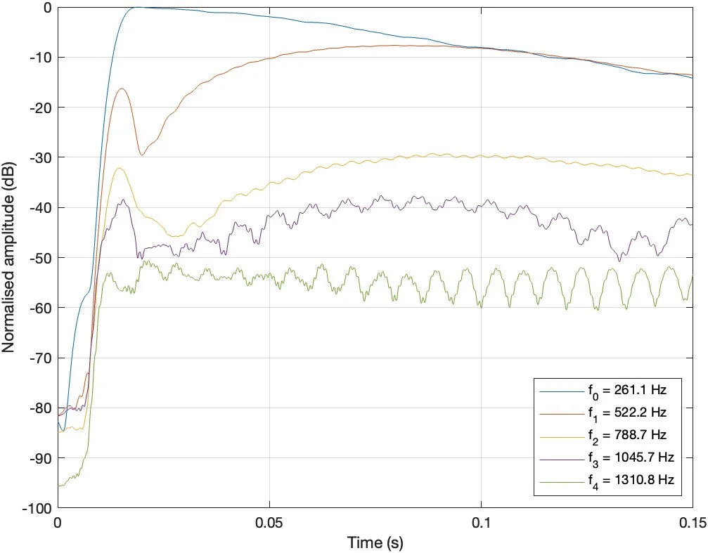
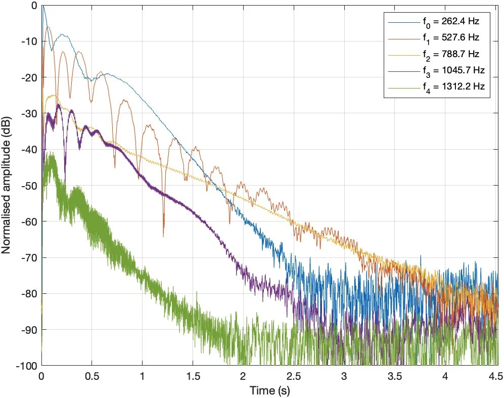
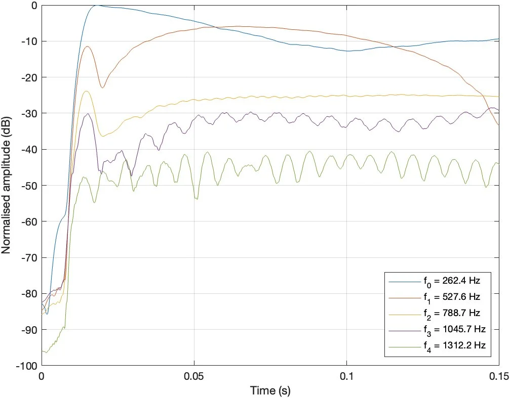
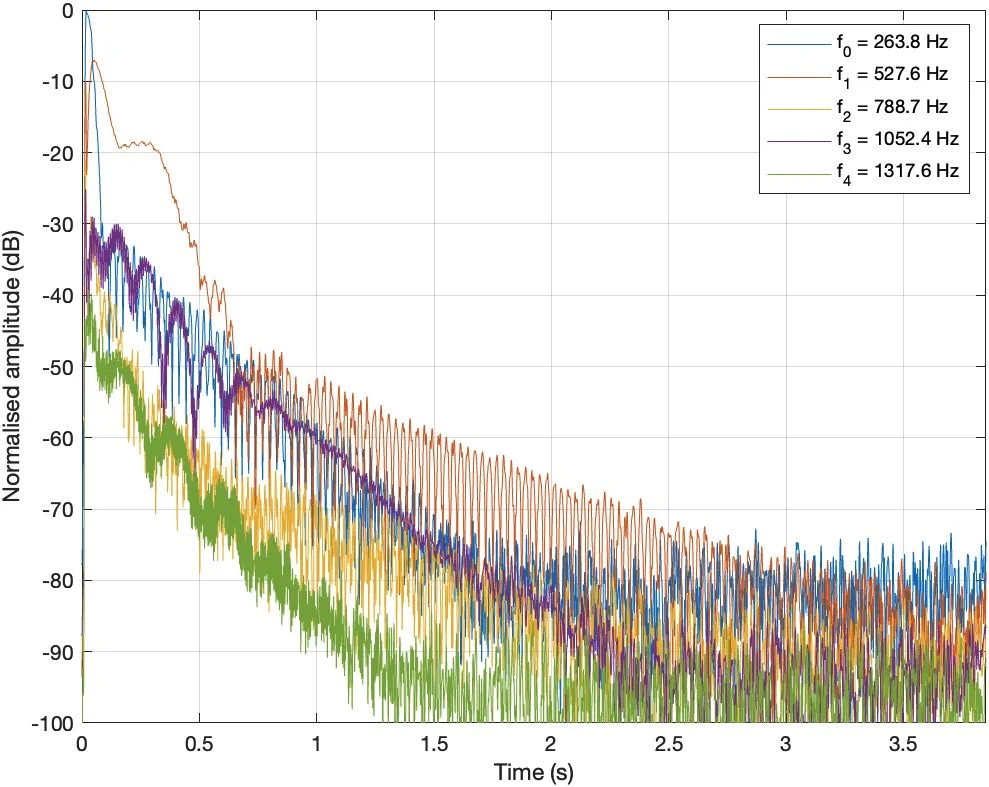
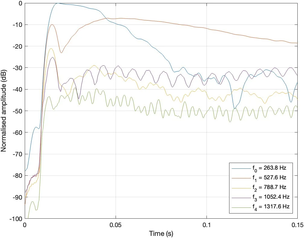
Figure 9: Normalised amplitude envelope for the first five harmonics of the struck note-field, extracted via the Hilbert transform, over their full length (left) and over the first 150 ms after impact (right), for all three recordings (top, middle, bottom).

4. Synthesis

Methodology
Based on the previous analyses, the recorded notes are synthesized in MATLAB using Time-Varying Partial Additive Synthesis (TVPAS) combined with Frequency Modulation (FM) synthesis.

The time-varying frequency of each partial is obtained from the instantaneous frequency, following from Eq. A.4, implemented for the discrete signal by cumulative summation. The amplitude envelope for each partial was obtained via Hilbert transform. To reduce data storage, the time-varying frequency and amplitude is stored only for the harmonics of the struck note-field. During synthesis, these characteristics are applied in a respective manner to the harmonics of indirectly excited note-fields. Hereby, it is assumed that all note-fields behave identical. The peak amplitude of each partial is derived from the PSD. Any partials possibly related to vibration of the shell (other than the note-fields) are disregarded.

The advantage of this hybrid synthesis method is the simplicity of additive synthesis, combined with the temporal accuracy of FM. With limited data extracted from the real instrument, many different sounds can be created. Furthermore, synthesis techniques deemed more advanced, such as physical modelling, are not trivial for this type of instrument due to its tuning process. Modelling the intricacies arising from the hammering process, which have a crucial influence on a note-field’s tuning, would require such a high level of detail that it might become computationally expensive and impractical to implement.

The main disadvantage is the need to store the time-varying frequency and amplitude for each harmonic of the struck note-field. However, these signals vary at relatively low rate and can be downsampled to a lower sampling frequency, significantly reducing the size of the stored data. In the transient phase of the sound, frequency and amplitude change at the fastest rate. Therefore, this part of the synthesized sound is most prone to artefacts due to downsampling.

Currently, the synthesis module enables for adding vibrato, tremolo and changing the pitch of the played sound. Pink noise and randomisation to the amplitude envelopes are added to increase realism.

Further improvements could include increasing the resolution of the resampled instantaneous frequency and amplitude envelope for the transients of the partials. Implementing the possibility to modify the amplitude envelope (e.g., stretching or shortening) might open up creative possibilities.

A diagram of the synthesis method is shown in Figure 10.

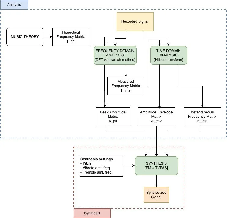
Figure 10: Diagram of the applied synthesis method.

Results
Figure 12 and 13 show respectively the PSD and spectrogram of all three notes, for both their recorded and synthesized version. Each synthesized signal comprises up to fifteen harmonics per note-field, limited to those partials identified in the recorded signal, together with the Helmholtz resonance. Harmonics of different note-fields coinciding in frequency were rendered only once. Pink noise and a random scaling of at most ±2 % applied to the amplitude envelopes were included

A notable feature is the reduced power for high-frequency components in the synthesized signals. This trend shows for all tree recordings and is quantified in Table 3. This difference is likely caused by implementing both the peak amplitude and amplitude envelope in the synthesis stage. Because the PSD peak represents the energy of an entire frequency bin, it may not accurately reflect the true amplitude of the partial. Table 3 also shows that omitting the PSD-derived peak amplitude in the synthesis stage results in a reduction of mismatch between the recorded and synthesized signals. Subjectively, an increase in presence is experience when comparing the two sounds.

Table 3: Difference in PSD estimate (in dB/Hz) between recorded and synthesized sounds, with and without using the PSD-derived peak amplitude in the synthesis stage.

	Note	f0	f1	f2	f3	f4	f5	f6	f7
with	1	11.4	6.6	3.9	0.2	−2.2	−5.5	2.5	−4.5
	2	5.4	−0.1	−1.0	−3.5	−6.3	−17.8	−12.5	−11.6
	3	4.8	−0.1	−2.0	−5.8	−7.9	−26.2	−8.7	−18.3
without	1	11.4	6.5	6.6	4.0	6.4	−5.1	3.6	−3.9
	2	5.3	0.4	0.5	0.4	0.5	−13.2	−10.4	−3.2
	3	4.8	−0.6	−0.1	−2.9	−2.7	−20.2	−4.2	−12.4

Also, the synthesized sounds contain audible high-frequency artefacts near the end of each note (which is masked by the added pink noise). These artefacts arise from the Hilbert transform applied to the filtered signals: as the amplitude of the partials approach the noise floor, the signals become broadband causing the Hilbert transform to introduce noise to the instantaneous frequency. Further smoothing of the Hilbert-derived time-varying signals may resolve this issue. Another solution would be adding noise to the synthesized signals; as demonstrated in the synthesis stage, the artefacts become barely audible when pink noise is introduced.

(a) note 1 synthesized without noise

(b) note 1 recorded

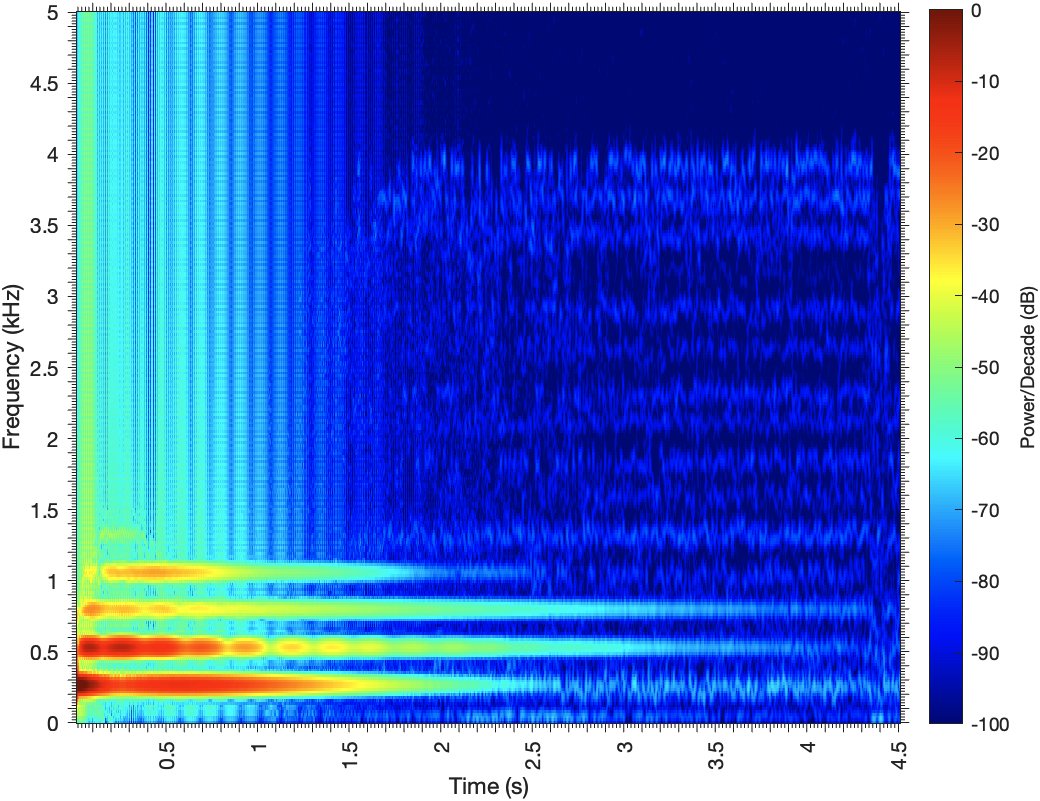
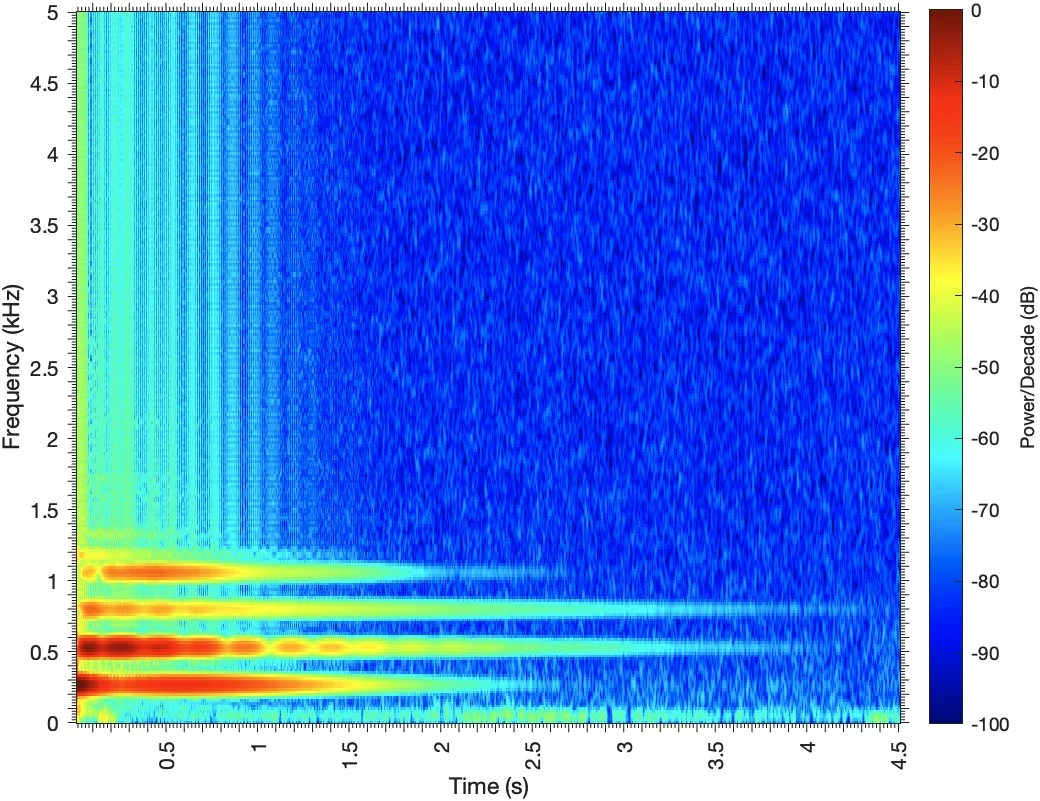
Figure 11: High-frequency artefacts arise from Hilbert transform.

(a)

(b)

(c)

(d)

(e)

(f)

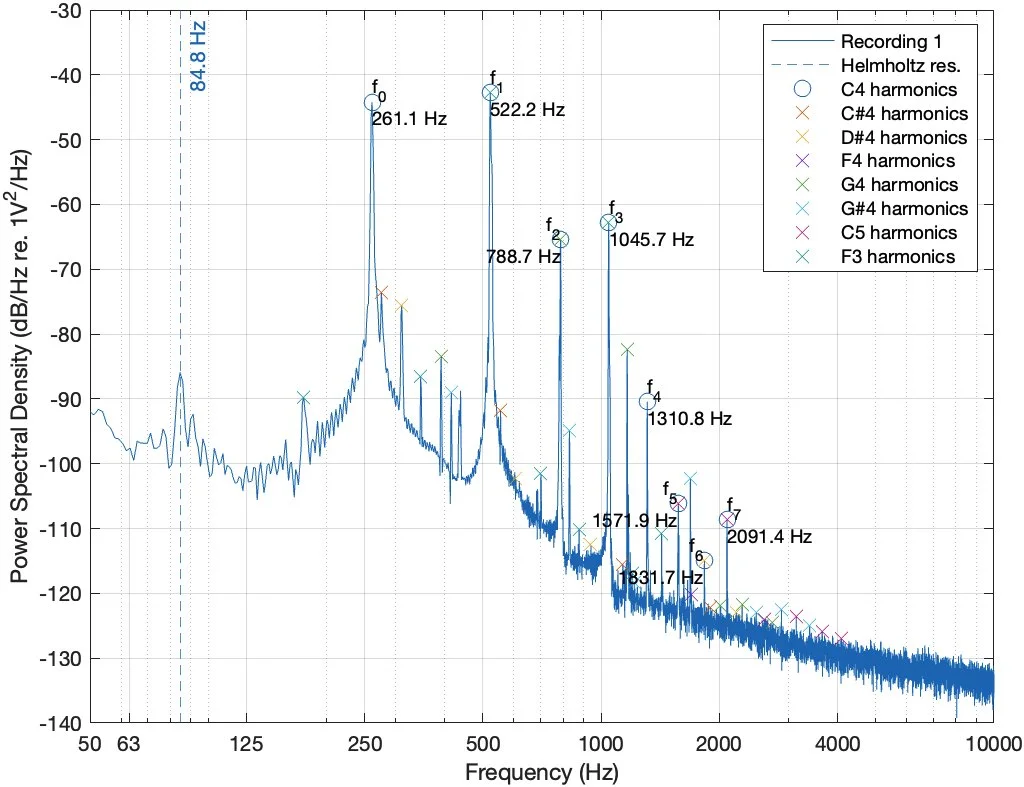
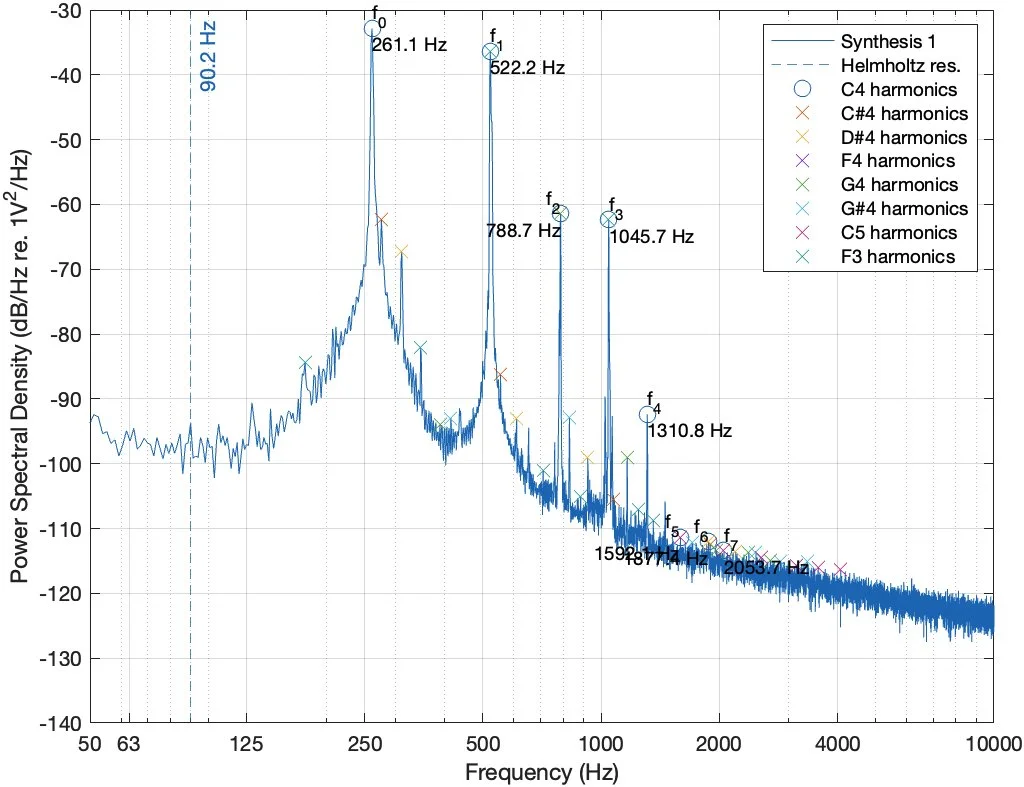
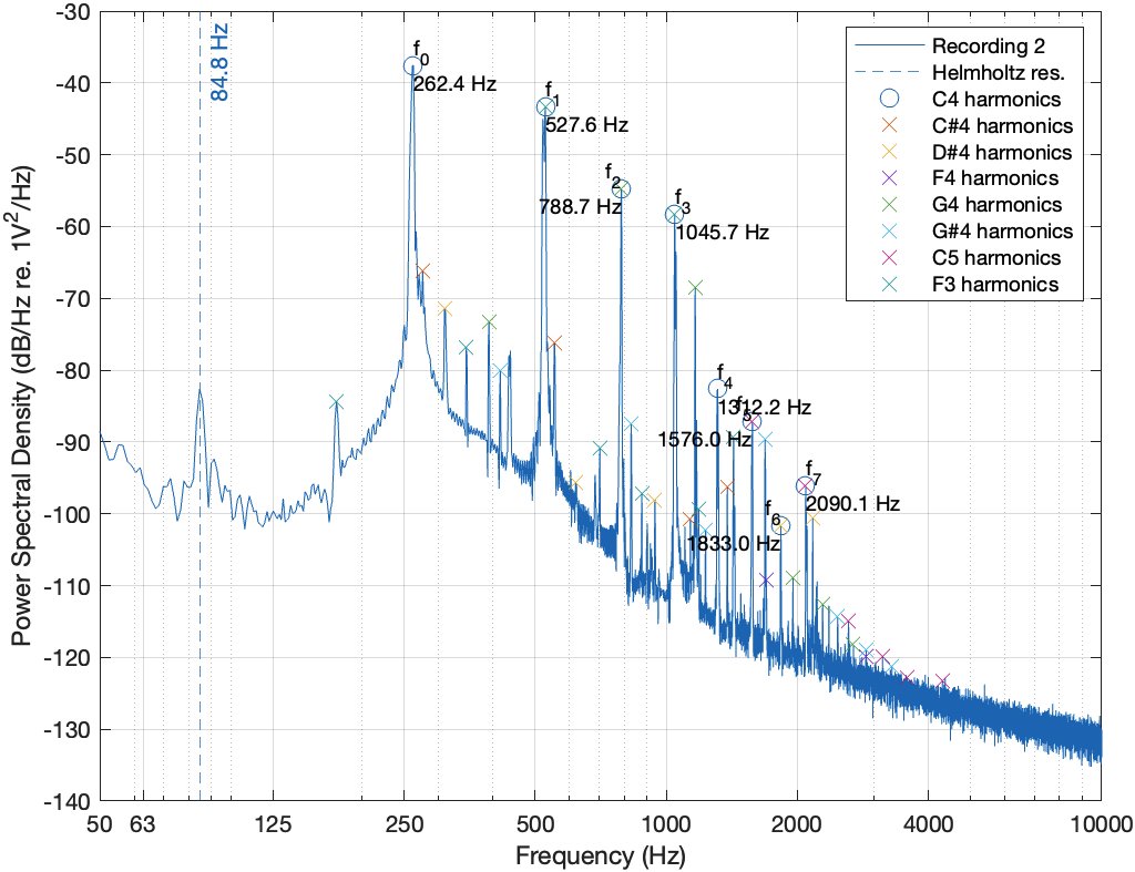
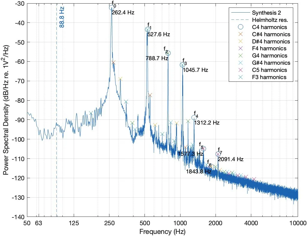
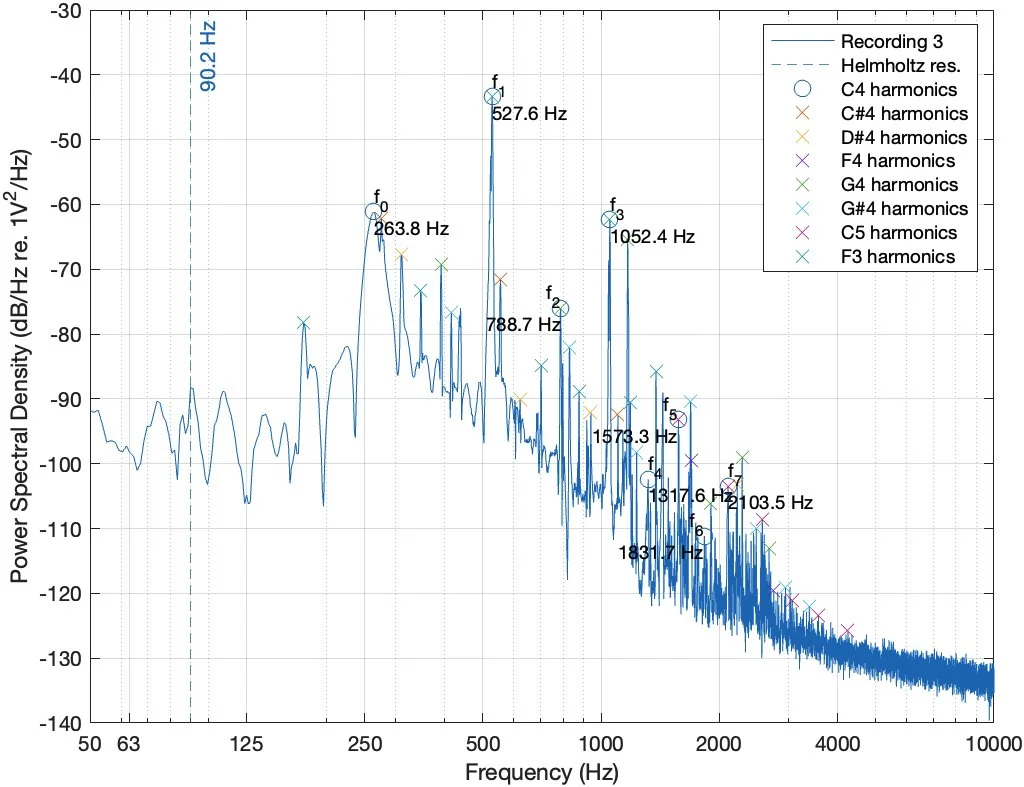
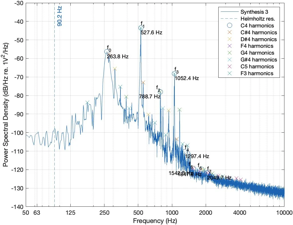
Figure 12: PSD estimates for recorded (left) and synthesized (right) versions of note 1 (top), note 2 (middle) and note 3 (bottom).

(a)

(b)

(c)

(d)

(e)

(f)

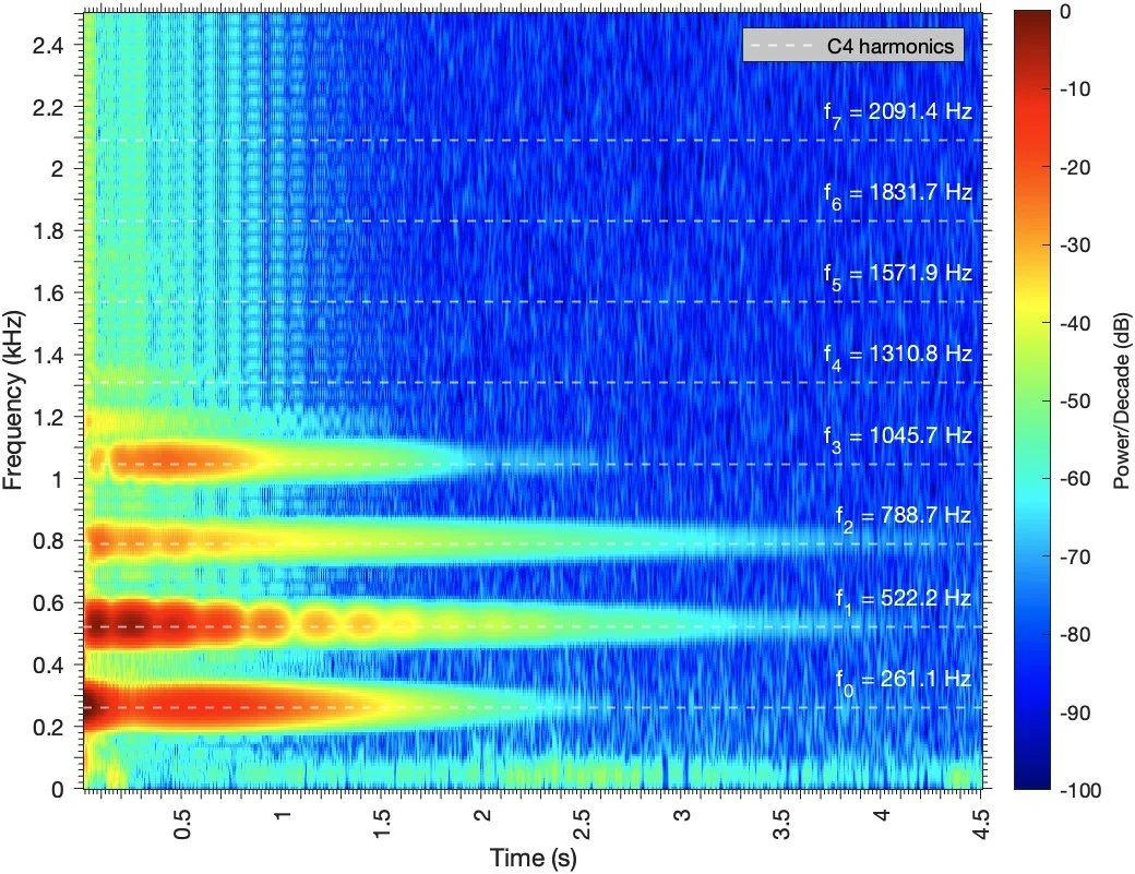
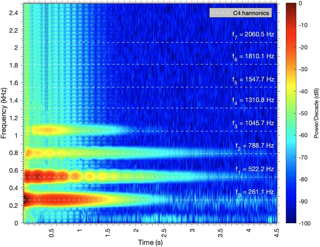
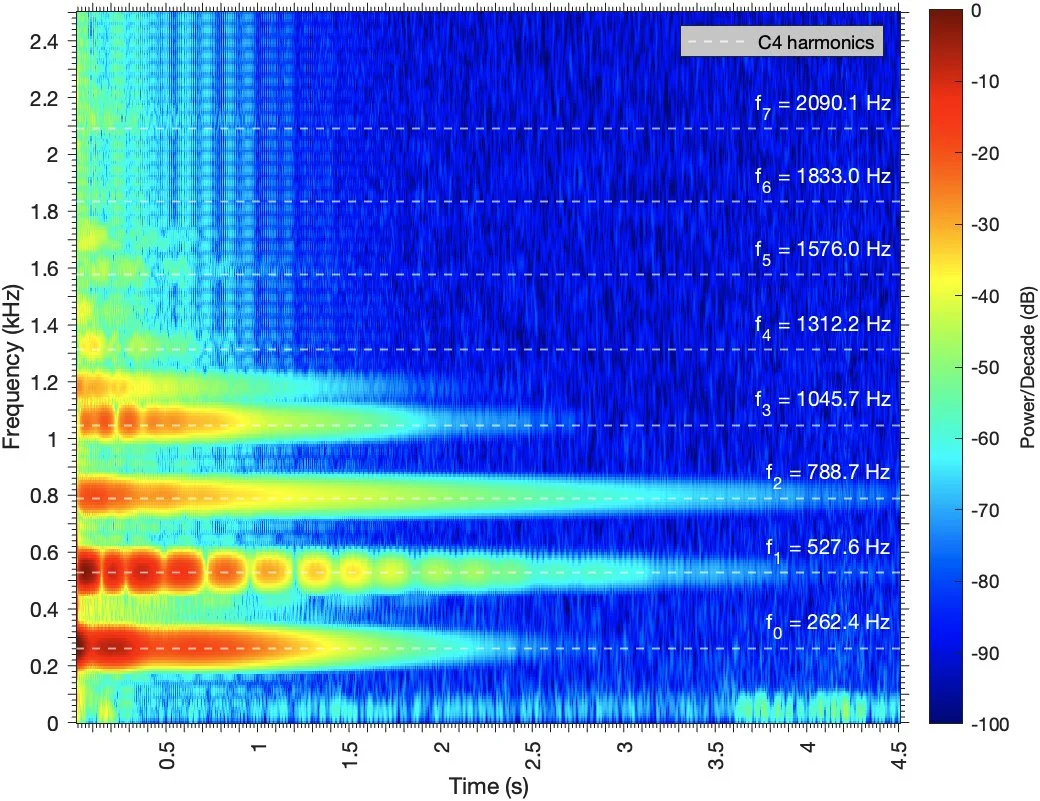
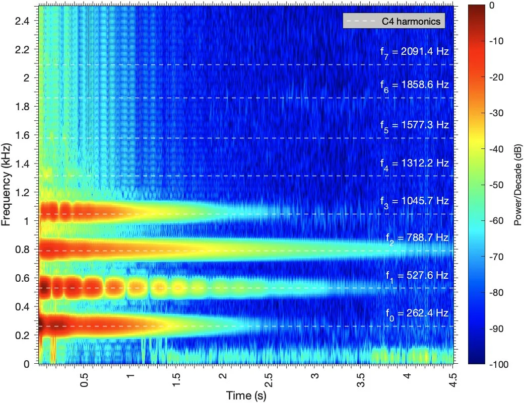
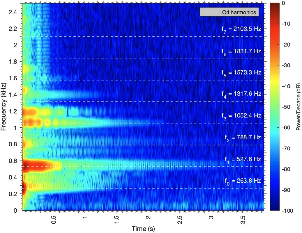
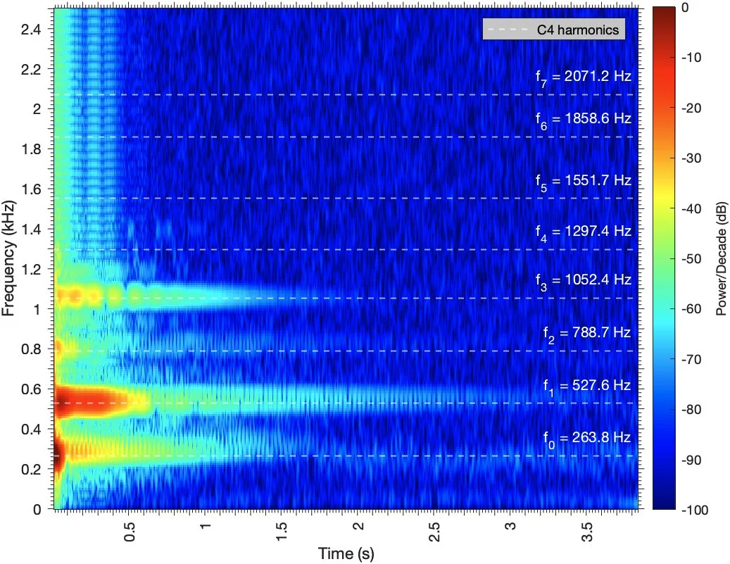
Figure 13: Spectrogram for recorded (left) and synthesized (right) versions of note 1 (top), note 2 (middle) and note 3 (bottom).

5. References

[1]        A. Morrison and T. Rossing, ‘MODES OF VIBRATION AND SOUND RADIATION FROM THE HANG’, Arch. Acoust., vol. 32, no. 3, pp. 551–560, 2007.

[2]        ‘List of idiophones by Hornbostel–Sachs number’, Wikipedia. Mar. 01, 2025. Accessed: Nov. 08, 2025. [Online]. Available: https://en.wikipedia.org/w/index.php?title=List_of_idiophones_by_Hornbostel%E2%80%93Sachs_number&oldid=1278343738

[3]        T. Rossing, A. Morrison, U. Hansen, F. Rohner, and S. Schärer, ‘Acoustics of the Hang: A hand-played steel instrument’, presented at the International Symposium on Musical Acoustics, Barcelona, Spain, 2007.

[4]        A. Morrison and T. D. Rossing, ‘The extraordinary sound of the hang’, Phys. Today, vol. 62, no. 3, pp. 66–67, Mar. 2009, doi: 10.1063/1.3099586.

[5]        F. Rohner and S. Schärer, Hang sound sculpture. Bern: PANArt Hang Manufacturing, 2013.

[6]        B. Singh and S. Chakraverty, ‘Use of characteristic orthogonal polynomials in two dimensions for transverse vibration of elliptic and circular plates with variable thickness’, J. Sound Vib., vol. 173, no. 3, pp. 289–299, 1994.

[7]        T. L. Reddy, P. V. P. Kumar, and A. Prajapati, ‘Modal analysis of an elliptical plate clamped along its boundary’, Int. Res. J. Eng. Technol., vol. 2, no. 9, 2015.

[8]        E. Alon, ‘Analysis and Synthesis of the Handpan Sound’, MSc by Research, University of York, York, 2015.

[9]        N. H. Fletcher and T. D. Rossing, The Physics of Musical Instruments, 2nd Edition. New York, NY: Springer New York, 1998. doi: 10.1007/978-0-387-21603-4.

[10]      S. Y. Mahmud, F. Snigdha, and A. S. Rakin, ‘Development of a Novel Method for Automatic Detection of Musical Chords’, Sci. Model. Res., vol. 3, no. 1, pp. 15–22, 2018, doi: 10.20448/808.3.1.15.22.

[11]      M. I. Ltd, ‘Behringer | Product | ECM8000’. Accessed: Nov. 10, 2025. [Online]. Available: https://www.behringer.com/product.html?modelCode=0506-AAA

[12]      ‘pwelch - Welch’s power spectral density estimate - MATLAB’. Accessed: Nov. 11, 2025. [Online]. Available: https://nl.mathworks.com/help/signal/ref/pwelch.html

[13]      D. A. Bies, C. H. Hansen, and C. Q. Howard, Engineering noise control: theory and practice, Fifth edition. Boca Raton: Taylor & Francis, 2017.

[14]      ‘VOICEBOX’. Accessed: Nov. 10, 2025. [Online]. Available: http://www.ee.ic.ac.uk/hp/staff/dmb/voicebox/voicebox.html

[15]      J. Guðnason, G. Fang, and M. Brookes, ‘Epoch-Based Spectrum Estimation for Speech’, in INTERSPEECH 2023, ISCA, Aug. 2023, pp. 4274–4278. doi: 10.21437/Interspeech.2023-407.

[16]      ‘Hilbert Transform and Instantaneous Frequency - MATLAB & Simulink’. Accessed: Nov. 11, 2025. [Online]. Available: https://nl.mathworks.com/help/signal/ug/hilbert-transform-and-instantaneous-frequency.html

[17]      T. J. Cox and P. D’Antonio, Acoustic absorbers and diffusers: theory, design and application, Third edition. Boca Raton: CRC Press, 2017.

[18]      M. Brookes, ‘spgrambw: Plot Spectrograms in MATLAB’.

[19]      D. M. Howard and J. A. S. Angus, Acoustics and psychoacoustics, Fifth edition. Routledge, Taylor & Francis Group, 2017.

[20]      L. Cohen, Time-frequency analysis. Prentice-Hall PTR, 1995.

Annex A – Hilbert transform

The Hilbert transform allows for expressing a real signal s(t) as an analytic signal z(t) in its complex form [20]

$$z(t)=s\left(t\right)+j\widehat{s}(t)$$ (A.1)

where

$$\widehat{s}(t)=\mathscr{H}\left[s\left(t\right)\right]=\frac{1}{\pi }\int \frac{s\left(\tau \right)}{t-\tau }d\tau$$

denotes the Hilbert transform of the real signal s(t).

The analytic signal z(t) can be expressed in its polar form

$$z\left(t\right)=A\left(t\right)e^{j{\varphi }_i(t)}$$ (A.2)

with ϕ_i(t) defined as the instantaneous phase (in rad). From (A.2) follows that

$${\varphi }_i\left(t\right)=\arg \left(z\left(t\right)\right)$$ (A.3)

Substituting (A.1) in (A.3) yields

$${\varphi }_i\left(t\right)=\arctan \left(\frac{\widehat{s}\left(t\right)}{s\left(t\right)}\right)$$

The instantaneous frequency ω_i(t) (in rad/s) is defined as the time derivative of the instantaneous phase ϕ_i(t), thus

$${\omega }_i\left(t\right)=\frac{d{\varphi }_i\left(t\right)}{dt}$$

or (in Hz)

$$f_i\left(t\right)=\frac{1}{2\pi }\frac{d{\varphi }_i\left(t\right)}{dt}$$ (A.4)

The amplitude envelope of the real signal s(t) follows from (A.2)

$$A\left(t\right)=|z(t)|$$